Reporting & Analysis
Nov 4, 2020
TLDR
You can use Google Sheets' query() function to filter data based on specific criteria, like finding days with over 1,000 impressions and over $10 spent. This involves two steps: first, aggregate the data into a new sheet using query() to simplify it, then run another query() function to filter the dates based on impressions.
With and without code.

The query() function is an extremely handy function within Google Sheets, that makes it incredibly easy to filter data within your sheet. Let's take three minutes to see how it works.
Case in Point: Pulling data from a Facebook Ads export based on multiple criteria
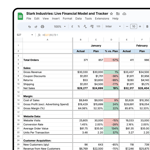
Let's say we have an export of data from Facebook Ads, something like the screenshot below and we want to answer the following question:
Which days did we receive more than 1,000 impressions and spent more than $10?
Sounds like a simple ask? It should be, but personally I don't think it is as simple as it sounds.
Here's the spreadsheet we will be working with:

Notice how there are multiple rows for every date. Unfortunately, the simplest way to do this is therefore a two-step process. This is how we will achieve our result:
Step 1: Pull the above data into a new sheet that aggregates the Impressions and Amount Spent data, using the query () function
Step 2: Run the query() function again to filter the dates according to impressions.

Step 1: Pull aggregated data into an interim sheet
We are going to add a new tab on the sheet and run this query() formula on cell A1.

The query() function works as shown in this Google article. It takes a little getting used to, but generally follows this format:
QUERY(data, query, [headers])
Once you run this function, you should get this result on your new tab.

Here, we have managed to aggregate the impressions and amount spent by each date. You can see that we now have one date per row. This is going to make our next step easier.
Improve your DTC game. Sign up for weekly tips.
Step 2: Run the query() function again to only show the rows with more than 1,000 impressions
This time, we are going to run a simpler query with two criteria.

This is going to look at your new sheet from the previous step, import all the three columns but only if they match the two conditions. This should give you the following result.

You're done! See how all the impressions are greater than 1,000 and amount spent is higher than $10?
Note: This process assumes that your raw data is in the same sheet as your analysis sheet. If you want to import in the data from another spreadsheet, you will have to use a more complex mix of IMPORTRANGE and QUERY. Let's leave that for another day!
