Reporting & Analysis
15.12.2021
TLDR
You can filter data in Google Sheets using the FILTER function, allowing you to specify conditions for data extraction. For example, you can filter data based on a single condition, such as finding rows where a certain column's values are greater than a specific number. Additionally, you can apply multiple conditions using AND or OR logic to narrow down your data further.
Oftentimes after gathering and collating data onto a spreadsheet, we want to focus on important figures that are relevant to our analysis. To do that, we have to filter our data. Google Sheets allows us to do this with the built-in FILTER function. This function works when you specify the range of data you want to be filtered and the Google Sheets filter conditions. This post will walk you through some frequently-used filter formulas to get common analyses.
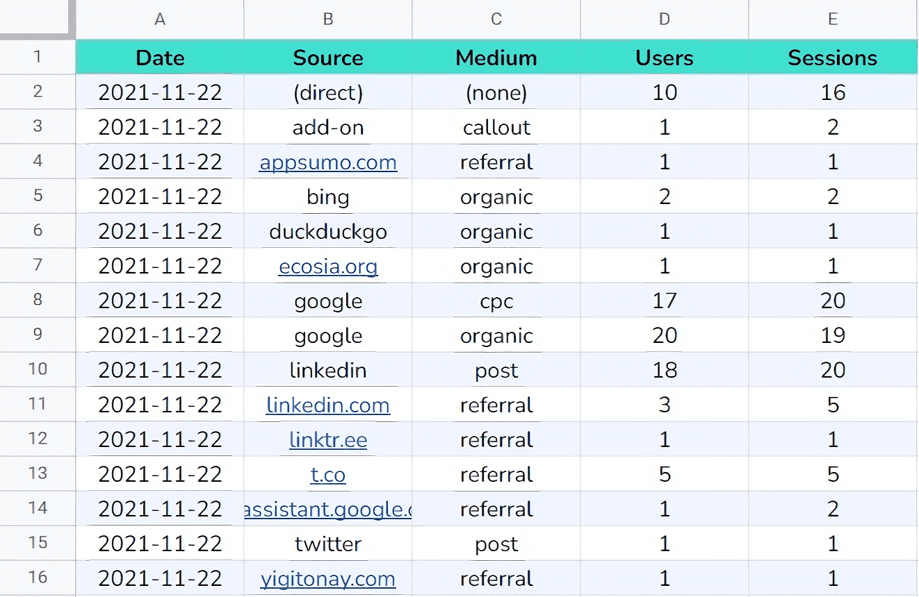
Let's say we want to analyze the traffic coming to our website with this dataset from Google Analytics.

Using FILTER with a single condition
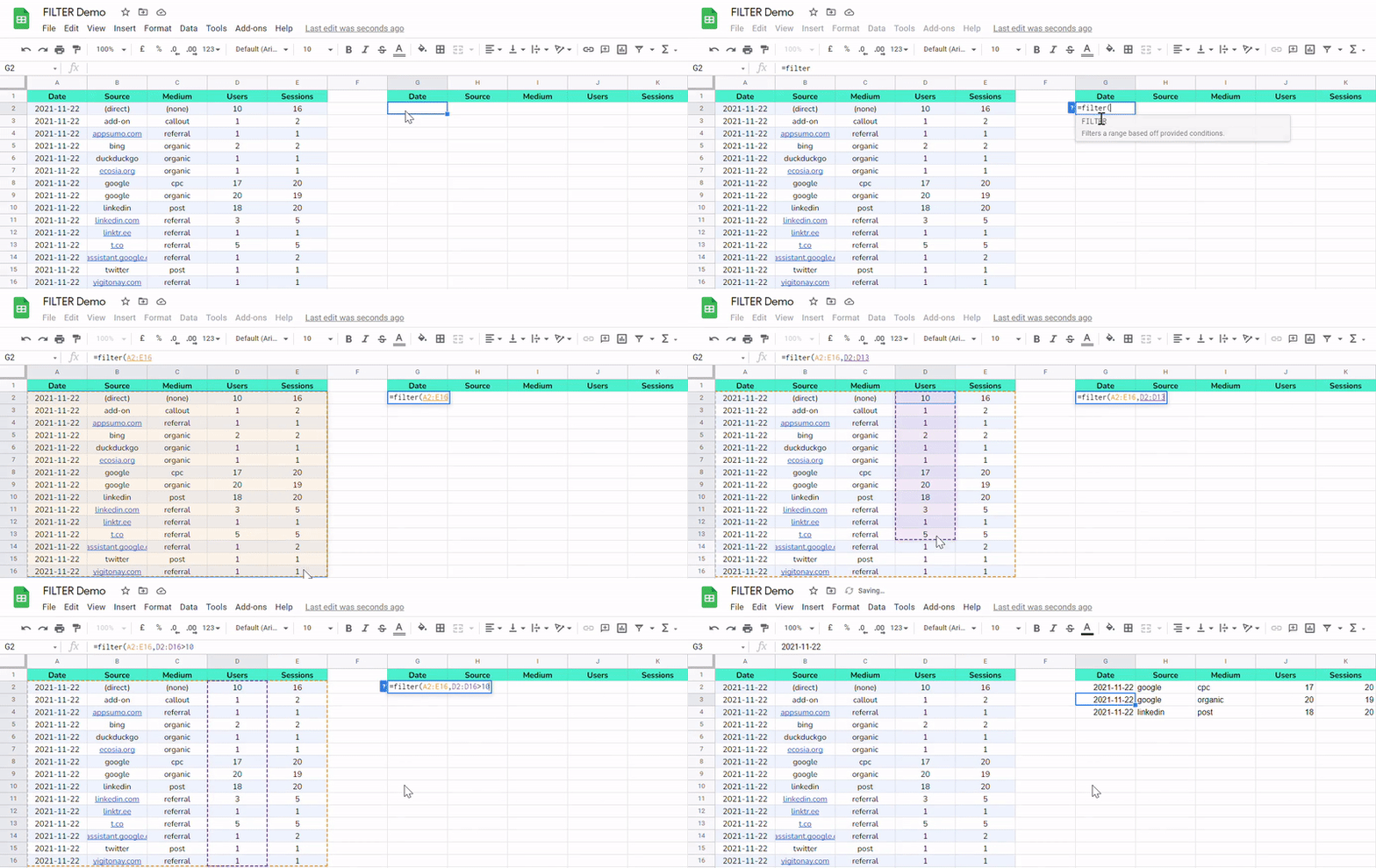
We want to find out which Source/Medium brings in more than 10 users. That is our condition.
First, we will specify the range of the column, Users then the operation:
D2:D16>10
Specify the range of data you want to filter and combine this with the condition formula above:
=filter(A2:E16, D2:D16>10)

And you're done!
Using FILTER with multiple conditions
The FILTER function doesn't just support one condition. It can filter multiple conditions and columns as well.
With multiple conditions, you have two options—do all the conditions have to be fulfilled or at least one? In other words, they are AND or OR conditions respectively.
First, we will explain the scenario with the AND condition.
Bringing back our original dataset, we now want to find out which Medium brought in more than 10 users from the Source, Google. This means the Users must be more than 10 and the Source must be Google. Each condition is separated by a comma:
D2:D16>10, B2:B16="google"
As you can see from above, we are filtering multiple columns. Similar to before, specify the range of data and the final filter formula will be:
=filter(A2:E16, D2:D16>10, B2:B16="google")

Notice how the data is only chosen when all the conditions are met.
Improve your DTC game. Sign up for weekly tips.
Next, we will explain the scenario with the OR condition.
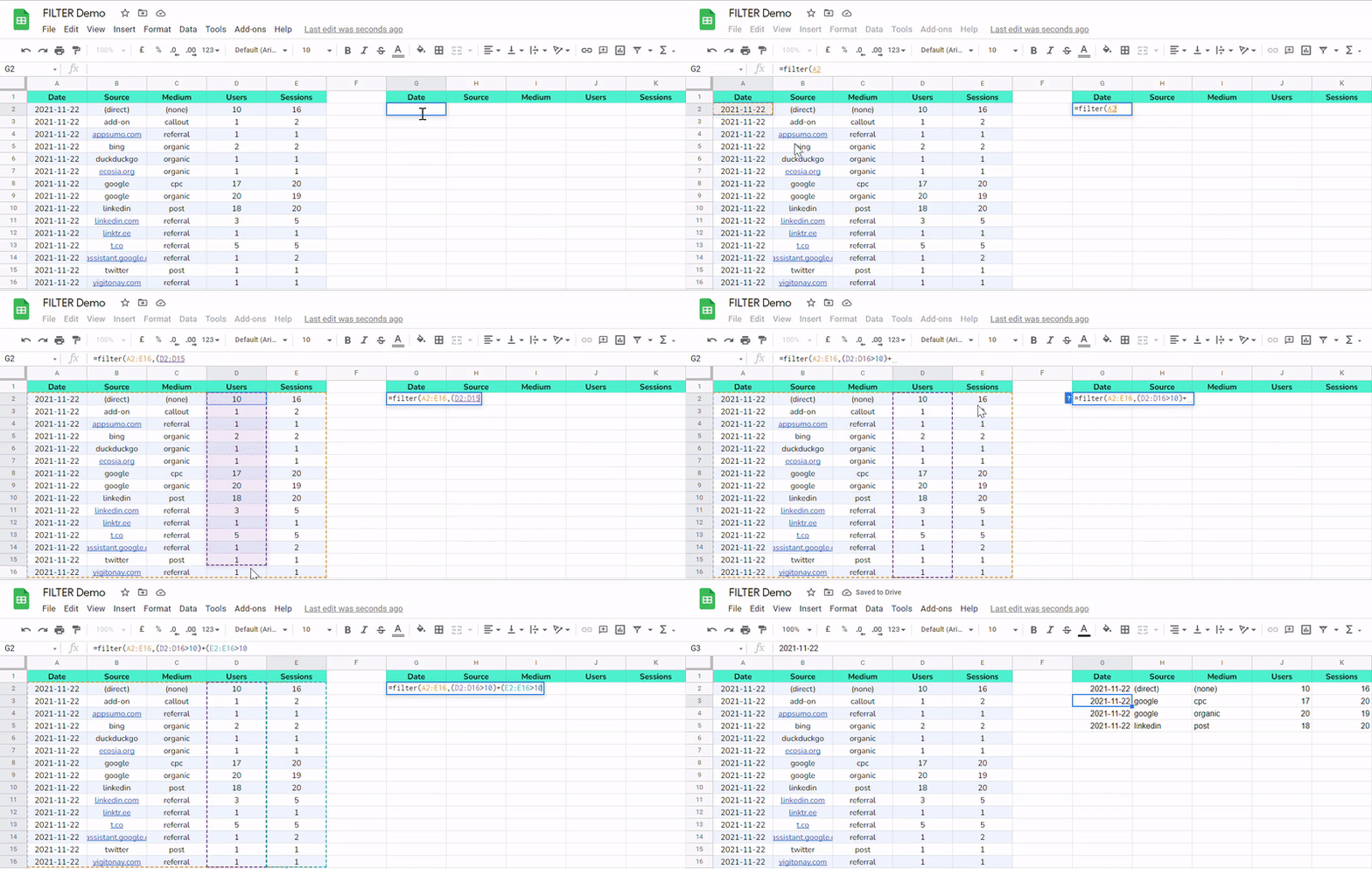
This time, we want to find out which Source/Medium brings in more than 10 users or more than 10 sessions. The formulas are now written differently—they are separated by brackets and the plus sign instead:
(D2:D16>10)+(E2:E16>10)
That will make the complete formula:
=filter(A2:E16, (D2:D16>10)+(E2:E16>10))

As mentioned earlier, the row of data will be selected once either condition is met.
Having just one or two conditions is easy to convert into formulas, but what if you have much more complicated operations?
Christabel Wong
About the Author

