Reporting & Analysis
08.03.2022
TLDR
You can easily transpose rows into columns in Google Sheets using two methods: Paste Special and the TRANSPOSE function. With Paste Special, select your data, copy it, choose a destination cell, right-click, select Paste Special, and then Paste Transpose. This method creates a static copy of your data. Alternatively, for a dynamic approach, select your destination cells, enter the formula "=TRANSPOSE(A1:B11)" (adjusting the range as needed), and press Enter. This automatically updates when the original data changes.
Google sheets is used extensively for businesses. These are free, easy to use, and accessible resources for businesses today. These spreadsheets stimulate transparency, and collaboration in a network. We often use Google tools such as Google Docs, sheets, slides and forms in the Google drive for day-to-day business tasks. These free cloud-based services efficiently make data more transparent and helpful in decision-making for businesses.
Google sheets are used to record day-to-day transactions, allowing users to enter, edit, organize, and analyze information. Multiple users can collaborate by using Google sheets as they can access, edit, and format files at a time, and changes are trackable by a revision history. Let’s review the simple and orderly solutions to convert (transpose) rows to columns, and vice versa in Google Spreadsheets, with examples.
What is transposing data?
When using Google Spreadsheets, you may sometimes need to convert rows into columns. But you don’t need to do this manually. To perform this specific task, we utilize a useful feature of Google sheets called Transpose. As the name implies, transpose means to rotate or interchange (in this case, data or information).
Transpose is a technique that creates a new data file in which the rows are switched to columns and columns are switched to rows.
Before you begin converting rows into columns, you need to have a table filled with data in a Google Spreadsheet. To do this, open Google Spreadsheets. You will be given two options for Personal or Business use. You can choose any one of these or Business use to gain extra security and more user controls.
After logging in an empty spreadsheet will appear on your screen. Fill the sheet with the required data.
Next, I will show you two great ways to transpose or convert rows into columns in Google Sheets:
Using Paste Special
Using the Transpose function
How to use paste special?
Paste Special is a simple way of converting rows to columns. Suppose you have the following dataset:
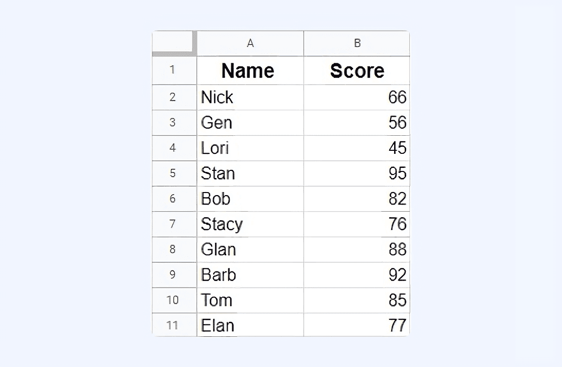
When you transpose this data, you will have the names in one row, and the score in another row below it.
Follow these steps to convert rows to columns in Google sheets:
Select the data that you want to convert or transpose.
Copy the data by clicking right and select copy or use the keyboard shortcut Control + C.
Select the cell where you want to drop the transposed data.
Right-click and select Paste Special, click on Paste Transpose.
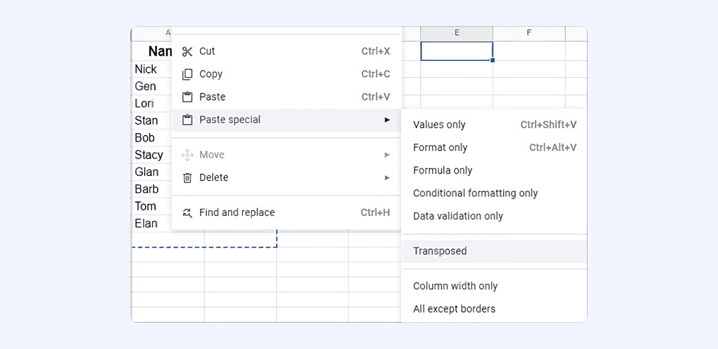
And you are done!
You will see that this has transposed the dataset.
Note that the data formatting is not done yet. You will have to copy its formatting separately. In addition, the data you transported is static. This indicates if the data changes, you will need to repeat above steps to get the latest transposed data.
How to remove the original data
Now that you’ve transposed your rows into columns or vice versa, you still have the original data where it was. Even if you use the Cut action instead of Copy in Step 2 mentioned above, that data remains. You can easily remove it by using one of the following two ways:
Select the cells containing the original data and hit the Delete key.
Drag through the removable columns. Right-click or click the arrow next to a column header and click Delete columns X – X.
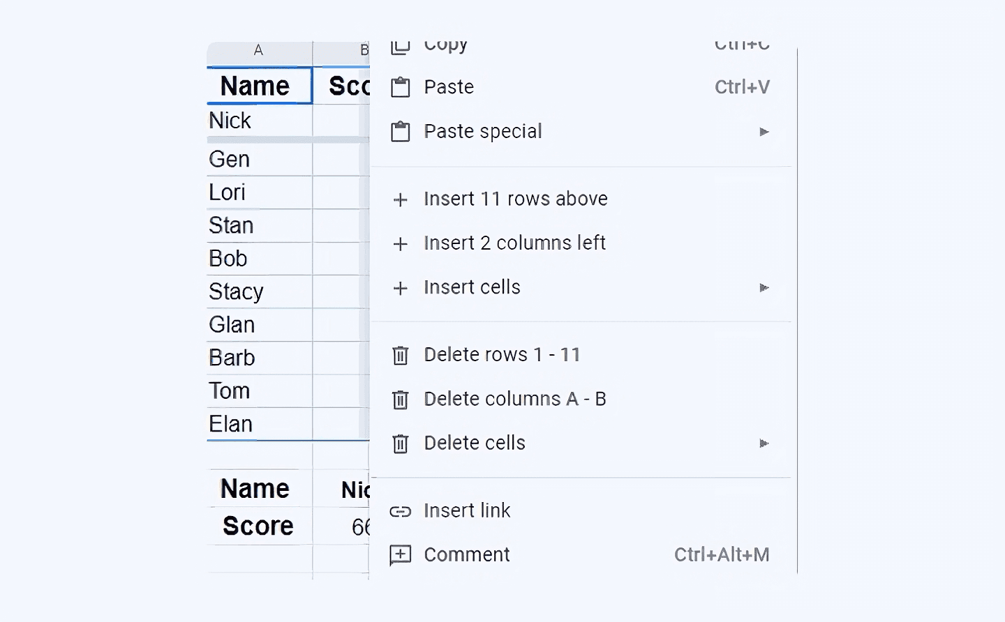
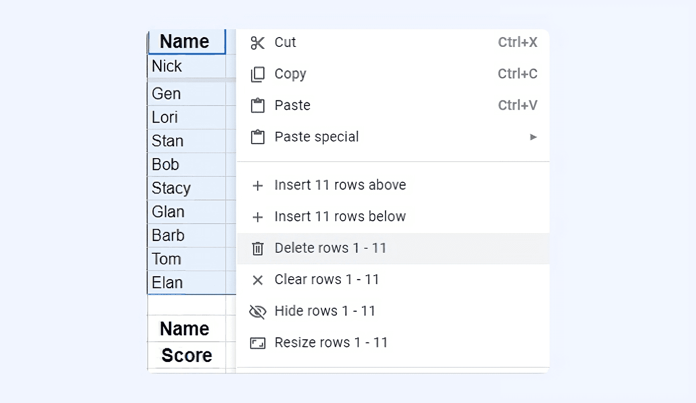
You may also be able to remove rows. But be sure your converted data doesn’t get affected.
● Drag through the removable rows, right-click, and click Delete rows X – X.
How to use the TRANSPOSE function?
In case you want to save a lot of effort and time, you need to make it dynamic, or automatic. To get dynamic data, use the TRANSPOSE function.
Again, let’s suppose we have the same dataset as shown below:

Follow these steps to transpose data using the TRANSPOSE function:
Select the cells where you want the data to be transposed or converted.
Enter the formula: =TRANSPOSE(A1:B11)
Press Enter.
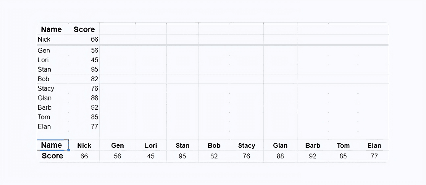
This would transpose the data instantly.
Google sheets can automatically sense if there is already some data in the cells that are to be used for this conversion, you will get a #REF! Error.
Also remember that you cannot delete a part of the array of the converted data. You will have to delete the entire dataset.
Improve your DTC game. Sign up for weekly tips.
How to convert multiple rows to columns in Google Sheets?
Suppose you have a list of items in a column, for example column A, and you want to transpose every n rows of this column to n columns at a time, then use the formula:
=INDEX($A:$A,ROW(A1)*N-N+COLUMN(A1))
Simply replace the “N” in the above formula with the number of rows you want to transpose at a time. So if you want to transpose every 5 rows, replace “N” with 5, so your formula will be:
=INDEX($A:$A,ROW(A1)*5-5+COLUMN(A1))
Copy this formula to the first cell of your transposed or converted table, then drag it out to copy it to the rest of the cells in the sheet.
How to convert rows to columns from one Google Sheet to another?
If you want to transpose data from a different sheet, you can again use the TRANSPOSE function. You will need to specify the name of the sheet from where you want to bring your data. So if you have your data to be transposed or converted in the cell range A2:B6 in Sheet1, then you can fetch this data and transpose it like this:
=TRANSPOSE(Sheet 1!A2:B6)
The idea is to make things simpler, and easier. In the present era of technology and competence, staying updated and well-equipped is mandatory to survive for any business or individual. Keeping up with the regular use of Google sheets is undoubtedly a good idea.
Set up the layout of your Google sheets anytime and any way you want to make it look more presentable and appealing. Google Transpose features can be used to display your data in the best way possible to present your ideas to the targeted audience, and impress them.


